

1. INTRODUCTION: Mont Terri fault slip experiment and DECOVALEX-2019 Task B
2. Fluid flow model in PFC3D
3. Modelling minor fault activation (Step 2 modelling in Task B)
4. Simulation results and discussion
5. CONCLUSIONS
1. INTRODUCTION: Mont Terri fault slip experiment and DECOVALEX-2019 Task B
The topic of fault reactivation by fluid injection has gained a significant attention worldwide and led to many R&D projects trying to better understand the underlying physical mechanisms of fluid and fault interaction (Zang et al. 2014). Lately, there have been several experimental studies on fluid injection induced seismicity where fluid is injected directly into a stressed fault/fracture system and monitor and measure their dynamic response. In laboratory scale, Passelègue et al. (2018), Jia et al. (2020a, 2020b) conducted experiments to investigate the influence of stress state and fluid injection rate on the fracture reactivation. In tunnel scale, Guglielmi et al.. conducted fluid injection experiment on a critically stressed fault in the shale formations of Tournemire France (2015) and in the Opalinus formation in Mont Terri Switzerland (2017, 2020). Such experimental studies provided direct observations on the fracture/fault behaviors and served as important database for developing numerical modelling methods/codes and improving their predictive capability.
The Mont Terri fault slip experiment consisted of a series of controlled fluid injection tests conducted in the main fault intersecting the Opalinus clay formation at Mont Terri Underground Research Laboratory (Guglielmi et al. 2017, 2020). The experiment aimed at understanding the conditions for slip activation and stability of faults, and the evolution of the coupling between fault slip, pore pressure and fluid migration. The Mont Terri URL is located in the southern limb of the SW-NE trending Mont Terri anticline (fault-bend fold, Fig. 1(a)) and where the studied fault, although called the “main fault” because it is the most deformed zone intersected by the laboratory facilities, is a minor splay. The Mont Terri main fault “core” consists of a thrust zone about 0.8 to 3 m wide that is bounded by two major fault planes. The “Step 2” fault slip experiment corresponds to injection tests using the SIMFIP (Step-Rate Injection Method for Fracture In-Situ Properties, Guglielmi et al. 2014) probe straddle packer interval set across a secondary fault zone in the main fault hanging wall (See Test 37.2 m in BFS2, marked in Figure. 1(b)). The fault zone contains 12 striated planes most of them oriented from N030° to N060° dipping from 50 to 70°SE. Two fault planes N030°-12°NW at 37.2 m and N160°-13°SW at 38 m contain a ~cm thick scaly clay layer.
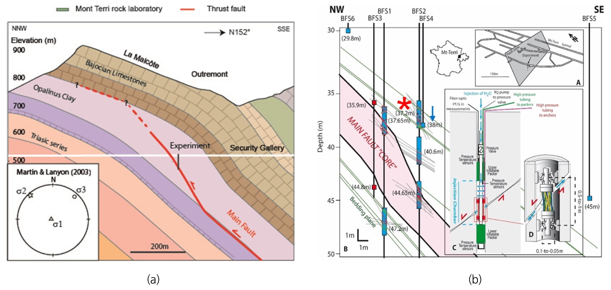
Fig. 1.
(a) Geological cross-section showing the main fault geometry and the experimental borehole location (Guglielmi et al. 2020). (b) A: 3D view of the Mont Terri fault plane with the location of the fault slip experiment, B: Simplified cross section of the main fault with the blue rectangles indicating the location of the packed-off section, C: SIMFIP test equipment setup, D: Schematic view of the 3D deformation unit (Guglielmi et al. 2017)
Based on that experiment, the Task B in DECOVALEX-2019 addresses how the change in permeability induced by the fault activation and the resulting fluid flow within the fault can be simulated. The aim was to support the understanding of the processes during fault activation, to develop, compare and validate models for activation of minor and major faults, including mechanical responses and associated changes in fault permeability (https://decovalex.org/task-b.html#collaboration).
Task B was conducted in the following three steps with increasing complexity:
∙Step 1: A benchmark calculation on activation of a single fault plane
∙Step 2: Interpretative modelling of observed minor fault activation
∙Step 3: Interpretative modelling of observed activation in a major fault
Seven research teams participated in Task B and their numerical methods/codes used in the modelling and how the fault structure was numerically represented are listed in Table 1. Park et al. (2018a, 2018b, 2020) used TOUGH2+FLAC3D coupled simulator and modelled the fault by zero-thickness interface elements in FLAC3D. Urpi et al. (2020) used FEM-based OpenGeoSys (Kolditz et al. 2012) and modelled the fault by finite-thickness solid elements. Nguyen et al. (2019) used FEM-based COMSOL Multiphysics software and modelled the fault by finite thickness solid elements. This study is one of those where distinct element method softwares (3DEC & PFC3D) were used.
Table 1.
Overview of the participating research teams and the modelling methods/codes and how they numerical represented the fault structure in Mont Terri URL
This paper presents application of Particle Flow Code 3D (Itasca 2019) in modelling of Step 2 minor fault activation experiment. The objective of the numerical modelling is to investigate if the currently developed fluid flow model in PFC3D could capture the field measurements of the Mont Terri fault slip experiment and to identify and discuss the limitations of the modelling method and issues for further development.
Numerical modelling of Step 2 minor fault activation experiment focused on simulating the STR1.1 injection cycle shown in Figure 2(a) (shaded region). The step-wise injection pressure evolution in the BFS2 borehole (Fig. 2(b)) is used as input in the numerical modelling (Section 3). The displacement, , is the anchor displacements of SIMFIP device (Fig. 1(b)) and have been filtered for estimated elastic deformation of the injection chamber and therefore represent the displacement caused by the deformation of the minor fault and the fractures intersecting the injection chamber. Fluid pressure at the monitoring point is at the borehole BFS4, which is located 1.5 m horizontally from the injection point at the borehole BFS2 (see Fig. 1(a) where the monitoring point at BFS4 is marked by blue downward arrow). The anchor displacements indicated fracture/fault deforms already during the first few injection pressure steps, with increasing displacement correlated with increasing injection pressure.
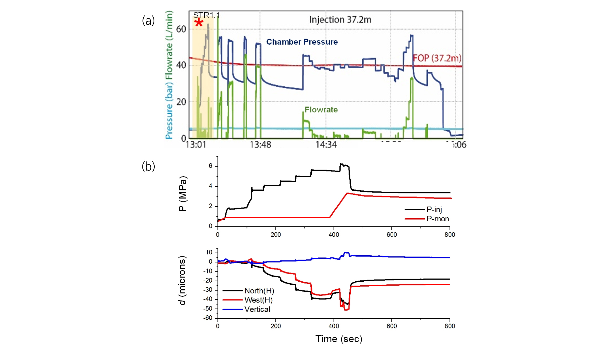
Fig. 2.
(a) Pressure and injection flow rate variations monitored at BFS2 injection interval (Guglielmi et al. 2017), (b) zoomed-in view of STR1.1 injection cycle (shaded-region) showing monitoring pressure evolution and displacements at injection interval
2. Fluid flow model in PFC3D
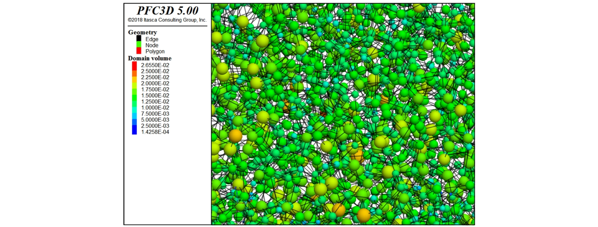
We used PFC3D (Itasca 2019). A fluid flow algorithm was developed and implemented in a 3D pore-pipe network model in a 3D bonded particle assembly. Flow of viscous fluid in the flow channel (pipe) is driven by the differential pressure between two ends of a pipe (a cylindrical tube), and it is modelled using the Hagen-Poiseuille equation, assuming that the flow is laminar. Figure 3 shows the 3D pore network model within a 3D bonded particle assembly, where the pores (spheres) are inter-connected by flow pipes (cylindrical tube). When a pressure gradient is applied, the volumetric pipe flow rate q (volume per unit time) is given by:
| $$q=\frac{\pi\;\bullet r^3}{8\;\bullet\;\mu}\frac PL$$ | (1) |
where, r is the hydraulic radius of the pipe (cylindrical tube), ΔP is the fluid pressure difference between the two neighboring pores, L is the length of the flow pipe, µ is the fluid dynamic viscosity.
The increment of pore fluid pressure ΔPf for a time step is computed from the fluid bulk modulus Kf, the pore volume Vd, and the net sum of the flow volume ∑q・Δt and the pore volume change due to mechanical effect ΔVd as:
| $$\triangle P_f=\frac{K_f}{V_d}(\sum_{}^{}q・\triangle t-\triangle V_d)$$ | (2) |
Using an explicit solution scheme, the fluid flow model alternates between applying the pore fluid pressure equation to all pores and applying the pipe flow volume equation to all pipes.
The flow into a pore due to a pressure perturbation ΔPf in the pipes surrounding the pore is calculated as:
| $$Q=N\frac{\pi・r_a^3・\triangle P_f}{8・\mu・L}$$ | (3) |
where, N is the number of pipes surrounding the pore, and ra represents the average hydraulic radius of the pipes surrounding the pore. The pipe length L is assumed to be 2 times of the average radius of two contacting particles (=). Equation (3) then leads to:
| $$Q=N\frac{\pi・r_a^3・\triangle P_f}{16・\mu・\overline R}$$ | (4) |
By equation (1), this flow volume Q causes a pressure response ΔPr:
| $$\triangle P_r=\frac{K_f・Q・\triangle t}{V_d}$$ | (5) |
For numerical stability, the pressure response ΔPr should be less than the original pressure perturbation ΔPf (i.e. ΔPr ≤ ΔPf). Therefore, from equations (4) and (5), a time step can be calculated as:
| $$\triangle t=S_f\frac{16・\mu・\overline R・V_d}{\pi・N・K_f・r_a^3}$$ | (6) |
where, Sf is the safety factor (= 0.5) which is to ensure numerical stability.
As shown in equation (1), the fluid flow in the rock model is represented by the pipe flow equation. A critical parameter, the pipe hydraulic radius r, is related to the macro-permeability of the rock model. In the case of an isotropic permeability, the Darcy flux q (unit of velocity) for a linear porous medium is given by:
| $$q=\frac k\mu\nabla P$$ | (7) |
where, the k is the permeability of the medium, and the ∇P=∆P/L. The flux can also be given by the average volume of flow contributions of all pipes within a control volume VC:
| $$q=\frac1{V_C}\sum\nolimits_{pipes}q_p・V_p$$ | (8) |
where, the qp is the flow flux in a pipe, which is calculated by dividing the volumetric flow rate in Equation (1) by the pipe cross-sectional area Ap = πr2p, Vp is the pipe volume.
Based on equations (1), (7) and (8), assuming that all the pressure differences across each pipe are the same for all pipes in a steady flow state, the relationship between permeability k and pipe hydraulic radius rp can be expressed as:
| $$k=\frac\pi{8・V_C}{\sum_{}^{}}_{pipes}L_p・r_p^3$$ | (9) |
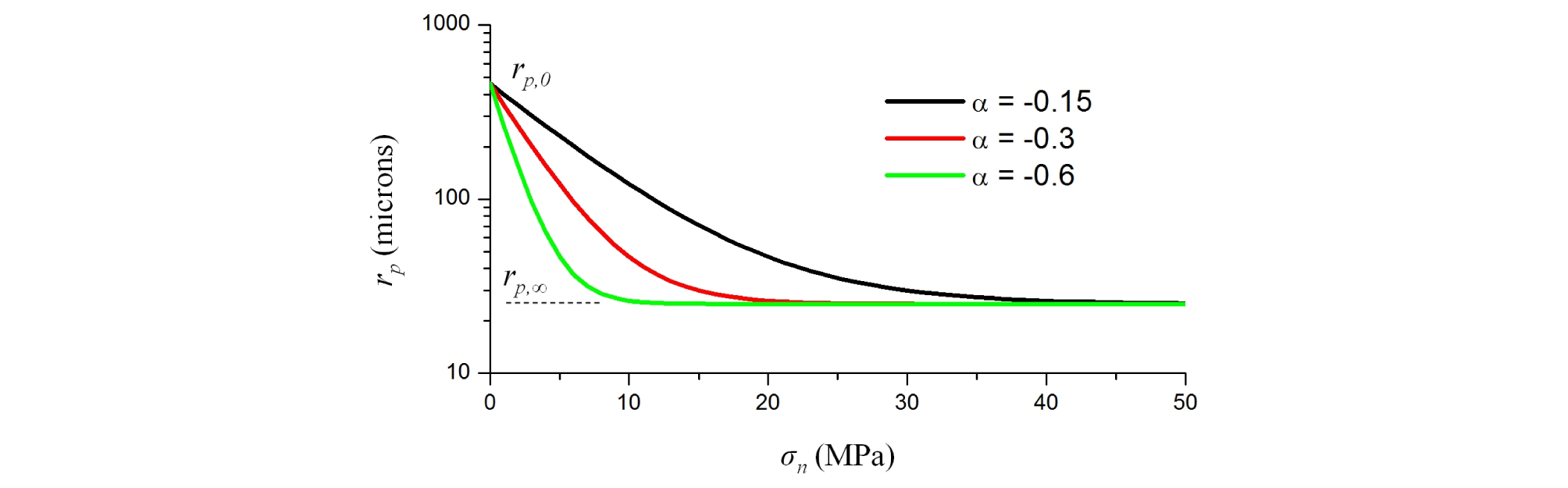
In the fluid flow model in PFC3D, we implemented a concept of stress-dependent permeability, which is to let the hydraulic radius of the pipe rp be dependent on the normal stress at the particle contacts (Hökmark et al. 2010; Yoon et al. 2014) as:
| $$r_p=r_{p,\infty}+(r_{p,0}-r_{p,\infty})\exp(\alpha・\sigma_n)$$ | (10) |
where, rp,∞ is the hydraulic radius of the pipe under infinite normal stress, rp,0 is the hydraulic radius of the pipe under zero normal stress, α defines the sensitivity of the radius decrease with increasing normal stress as shown in Figure 4. In this study, we used the α= -0.6. The two end members of the hydraulic radii, rp,∞ and rp,0, are determined by the permeability values given as user input:
permeability of unfractured/intact rock and permeability of fractured rock.
3. Modelling minor fault activation (Step 2 modelling in Task B)
The model setup for Step 2 modelling is shown in Figure 5. The model dimension is 20 × 20 × 20 m3. In the volume, particles with diameters ranging between 0.5 m to 0.6 m are randomly distributed. In total, 9103 particles are packed in the volume. The particles are then bonded at their contacts by the parallel bond model, of which the parameters are listed in Table 2. In addition, a fault is implemented with 65° dip. Stresses applied to the model are: 6 MPa in x-direction (Sx, perpendicular to the fault strike), 3.2 MPa in y-direction (Sy, parallel to the fault strike) and 7 MPa in vertical direction (Sz).
The particle contacts at the location of fault plane are assigned smooth joint contact model (Mas Ivars et al. 2011) (Fig. 5(b)), In such way, we modelled the fault structure similar to the nature where the fault zone is a combination of fault damage zone and fault core fracture as shown in the sketch in Figure 5(c) (Lin & Yamashita 2013). The fault core fracture is modelled by smooth joint contact model which is proposed and developed to overcome some of the limitations of PFC in modelling jointed rock mass behavior (Mas Ivars et al. 2011). The mechanical parameters of the smooth joint contact model for representing the fault core fracture are listed in Table 2.
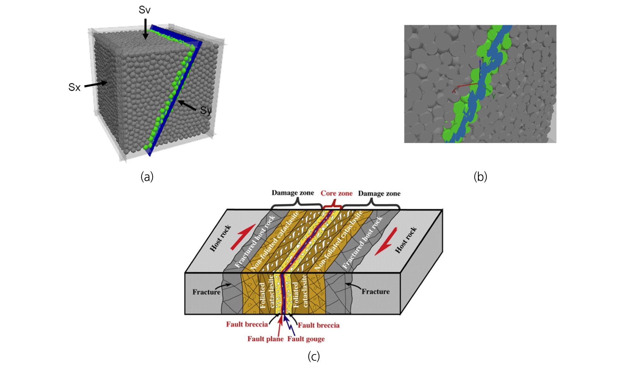
Fig. 5.
(a) 3D model geometry for Step 2 benchmark modelling, (b) close-up cross-section view of the fault zone, and (c) schematic model of a fault system composed of damage zone and core fracture (Lin & Yamashita 2013)
Table 2.
Values assigned to the parallel bond model and the smooth joint contact model
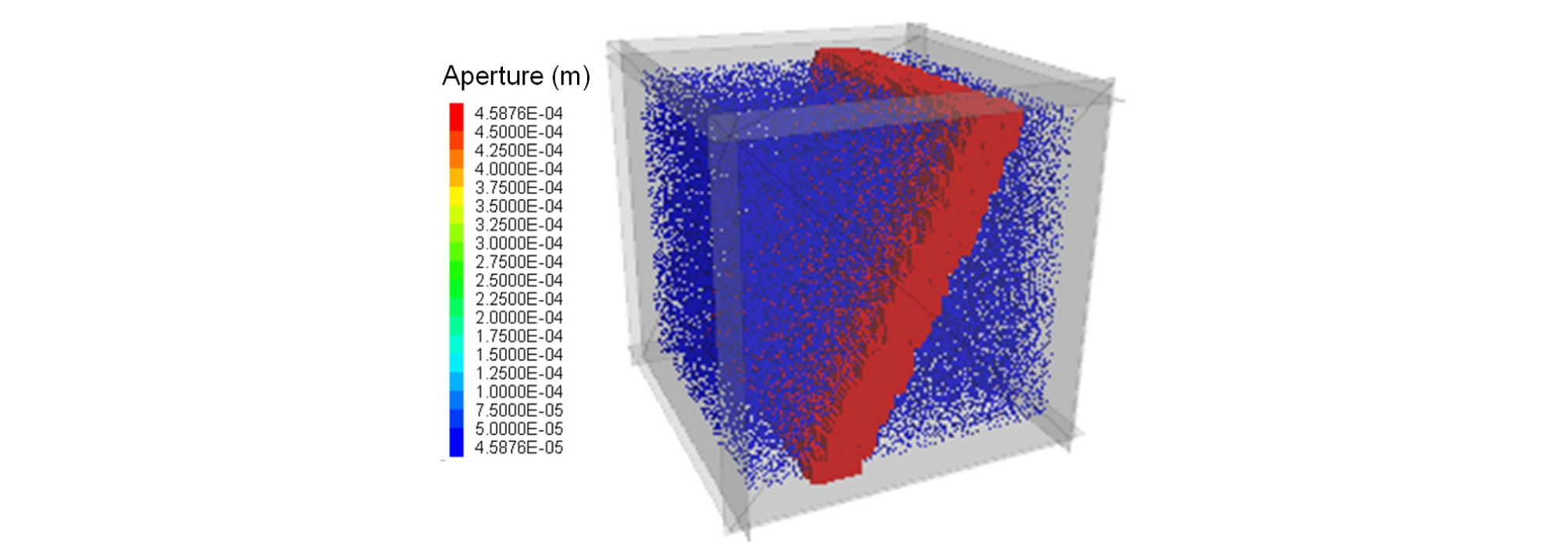
The host rock is assumed to be linear elastic and isotropic with a bulk modulus K = 5.9 GPa and a shear modulus G = 2.3 GPa, which represent average value of Opalinus clay formation at the Mont Terri URL. The host rock is considered impermeable, which is reasonable considering the very low permeability of Opalinus clay. In order to mimic such low permeability host rock, we assigned hydraulic permeability of 1e-18 m2 to the particle assembly in the host rock part. Fault permeability was programmed to be larger than the host rock by two orders of magnitude. The fluid flow algorithm was programmed to calculate the fluid flow channel aperture (pipe radius) based on the permeability given as user input using equation (9) and the aperture-stress relation using equation (10). The resulting aperture in the fault zone is 0.458 mm. Figure 6 shows how different the initial apertures are in the fault zone and in the host rock part. This is the starting model for the fluid injection simulation.
4. Simulation results and discussion
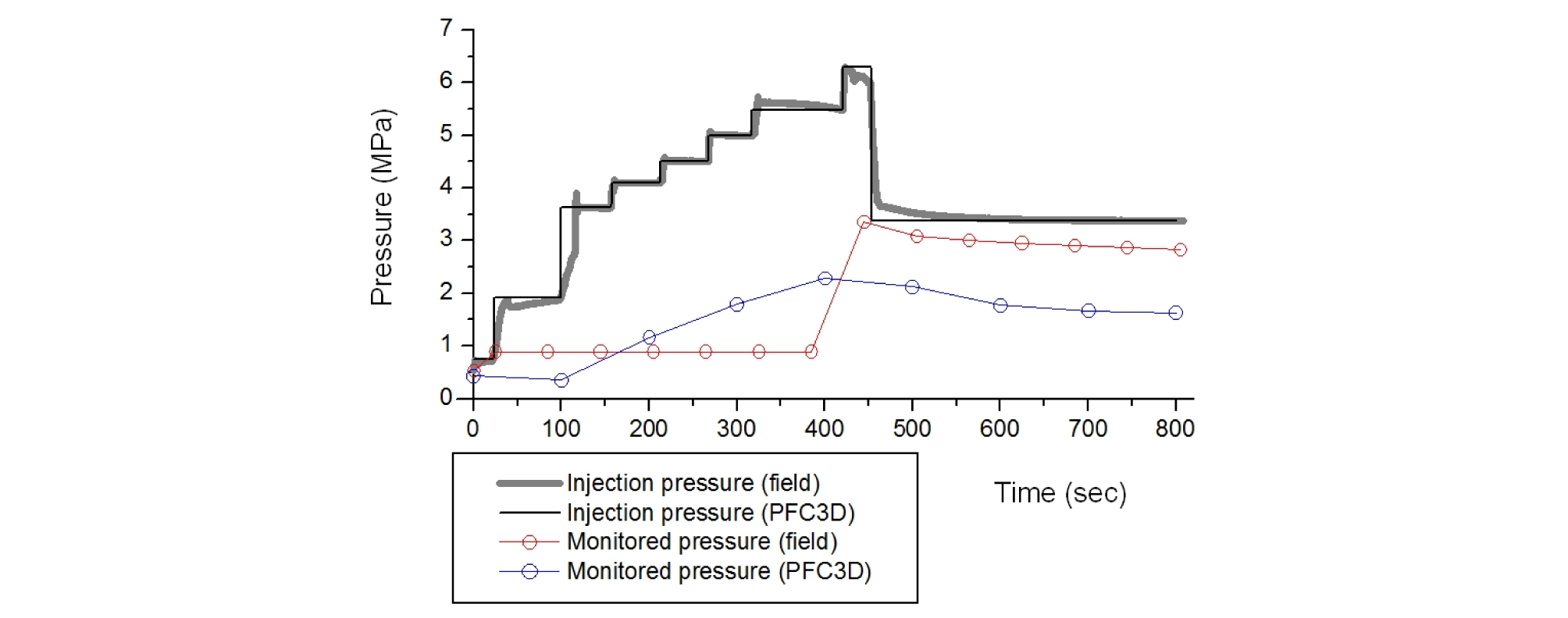
Figure 7 shows the temporal evolution of the injection pressure applied at the model center (black curve): injection location (0,0,0), and the fluid pressure evolving at the monitoring point (blue curve) which is located 1.5 m horizontally from the injection point. As the model was initially saturated with pore pressure of 0.5 MPa, the monitored pressure starts from 0.5 MPa. Unlike the field measurement (red curve), the simulated pressure shows a smooth increases with time. After 400 seconds, the monitored pressure starts decreasing even when the injection pressure is still increasing. This is due to the fact that the fluid migrates faster in the orientation of fault dip, and the fluid pressure registered at the monitoring location is also affected by such faster fluid migration. The simulated monitoring pressure did not show sharp increase as observed in the field measurement. The difference is probably due to the fact that the fault in the field experiment is narrower compared to the fault zone modelled. Also the clay fillings in the fault zone at the Mont Terri site could have acted as a fluid barrier from which fluid over-pressurized zone could develop locally in the fault zone. When the fluid over-pressure became large enough to break the fluid barrier, a significant amount of fluid migrated into the monitoring pressure location. Such behavior was not precisely simulated in the PFC3D modelling, and left as one issue for further study. However, we confirmed that the model is able to capture the overall behavior of the pressure evolution at the monitoring location induced by fluid injection.
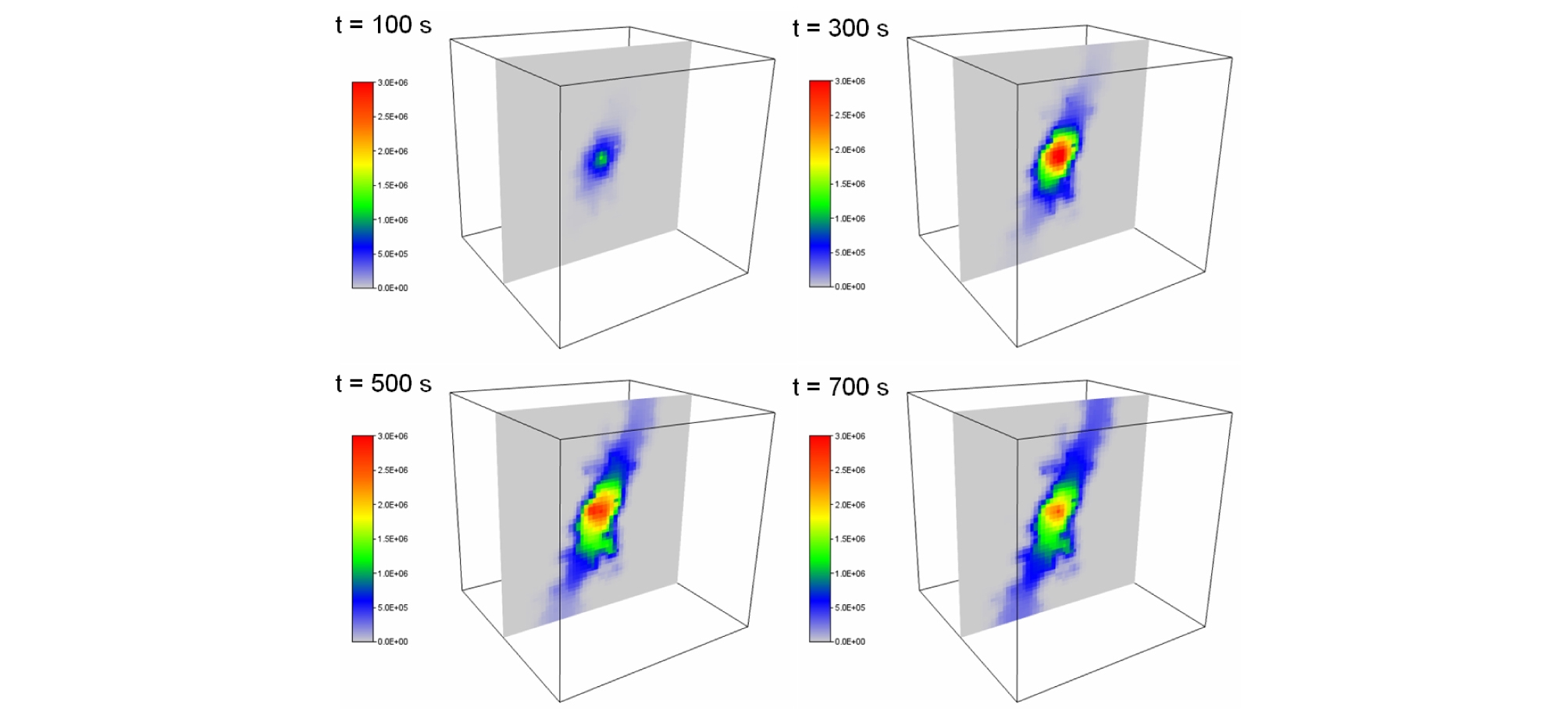
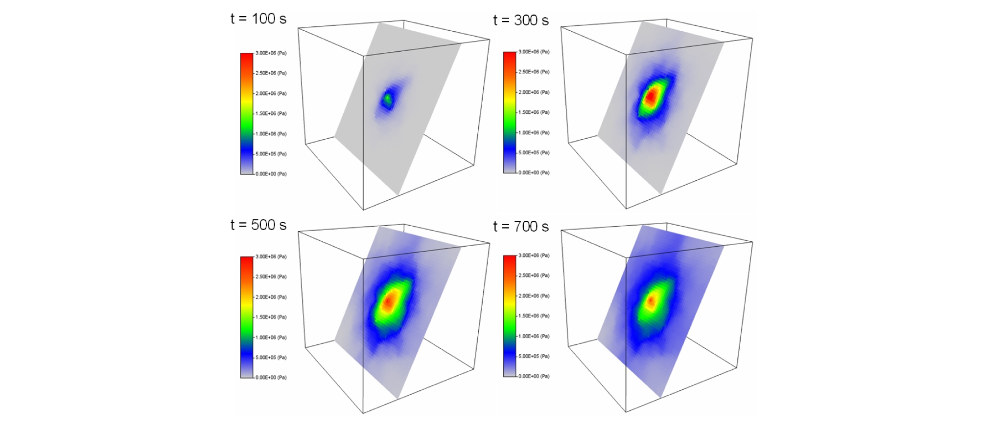
Figures 8 and 9 demonstrate how the injected fluid distributes in the fault zone over time. As the fault is modelled as a zone with thickness of 2 m, the fluid pressure propagates along the fault zone and very little fluid is migrating into the rock part due to its low permeability. This is visualized in Figure 8, which is a vertical cut section at the model center. Figure 9 shows the fluid pressure distribution on the core fault plane and it demonstrates that the distribution develops radially in general. However, the migration speed is slightly larger in the direction of fault dip (z-axis) compared to the migration speed in the direction of the fault strike (y-axis). This is due to the stress applied to the model, as the fluid flow channel aperture is programmed to be stress-dependent using equation (10). The fluid flow channels aligned parallel to the fault zone (in the orientation of fault dip) has larger apertures compared to those aligned parallel to the fault strike. In this modelling, the parameter α in equation 10 plays a significant role as it defines how the aperture should change by the stress state.
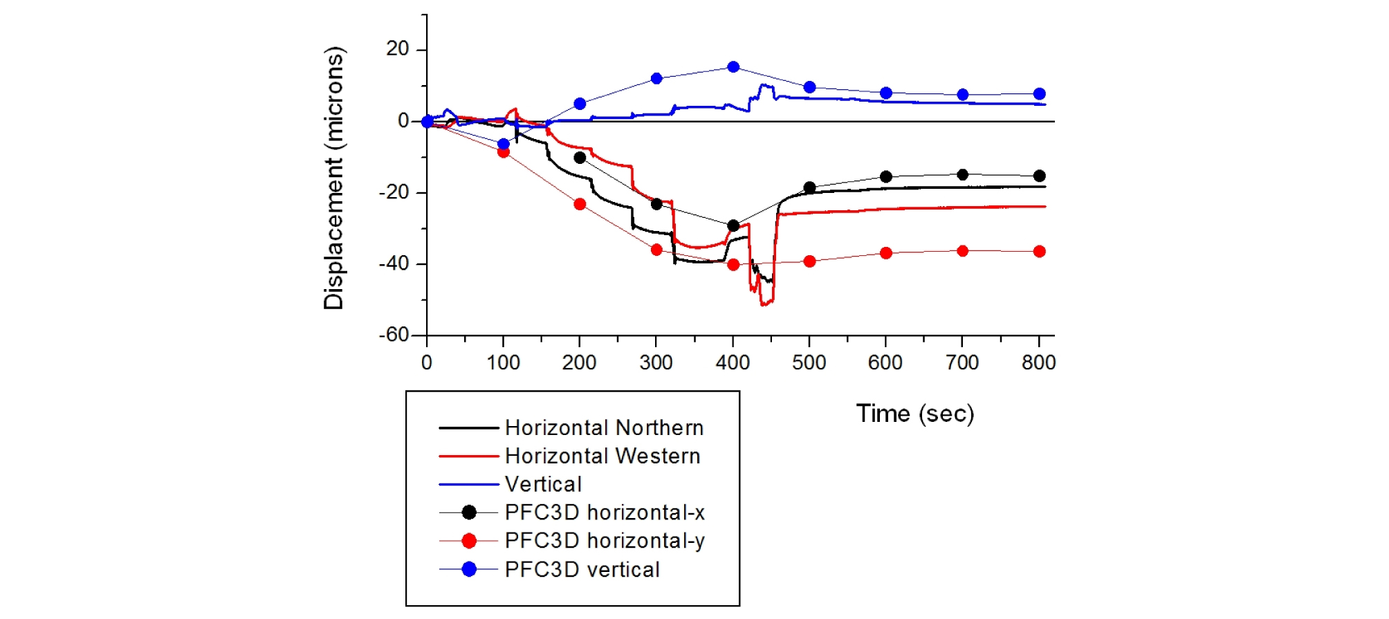
We also monitored the displacement results of the simulation. The field-measured displacements shown in Figure 10 correspond to anchor displacements monitored by SIMFIP device (two horizontal displacement: North and West, and vertical displacement) installed at the injection location. For PFC3D, the simulated displacement is calculated by reading the x, y, and z displacements of the smooth joint located closest to the injection point. As the anchor displacements are determined by calculating the upper and the bottom part displacement of SIMFIP device which is separated by 0.5-1 m, the data obtained from the smooth joint displacement reading was calibrated to properly take into consideration of this 0.5-1 m measuring interval of SIMFIP. The simulated results shown in Figure 10 are therefore after-calibration data. Due to technical difficulty, continuous recording of the displacement data was not allowed. Instead, the displacement data at the selected times were extracted from the PFC3D result files. Figure 10 demonstrates that the field measured displacements show step-wise increase as a direct response of the step-wise increase of injection pressure, whereas the simulation results show rather smooth evolution. Again, in the displacement evolution, the simulated results show partially matching behavior to the field measurement. However, we confirm that the overall behavior of the displacement evolution shows quantitatively matching results. A follow-up study is in progress where we try to mimic heterogeneous distribution of the clay fillings in the fault zone, and to monitor the displacement continuously. Such approach is tried by modifying the fluid flow algorithm so that the fluid flow apertures at the smooth joint contacts are assigned lower than the contacts in the fault damage zone. Also, the stiffness of the smooth joints can be heterogeneously distributed in the fault zone.
5. CONCLUSIONS
This study presents a fluid flow model in Particle Flow Code 3D, that joined in the Task B of DECOVALEX-2019 for simulation of the Mont Terri fault slip experiment. A 3D pore-network model was generated which is interconnected by fluid flow pipe by python/FISH programming and implemented in a 3D bonded particle assembly. Except that the model dimensionality is increased to 3D, the basic idea of fluid flow logic is same as that of Hazzard et al. (2002) and Yoon et al. (2004, 2017). We applied the 3D fluid flow model to simulation of fault slip induced by fluid injection, Step 2 minor fault slip experiment conduced at the Mont Terri URL site in Switzerland. In PFC3D modelling, we modelled the fault structure as a zone, with combination of damage zone and core fracture using the smooth joint contact model. The simulated results showed that the pressure evolution did not show a good matching with the field measurement. The modelling results showed pressure increase linearly with time, whereas the field measurement showed an abrupt increase associated with fault slip. We conclude that such difference between the modelling and the field test is due to the structure of the fault in the model. The modelled fault is likely larger in size than the real fault at the Mont Terri site. Therefore, the modelled fault allows several path ways of fluid flow from the injection location to the pressure monitoring location, leading to smooth pressure build-up at the monitoring location while the injection pressure increases, and an early start of pressure decay even before the injection pressure reaches the maximum. We also conclude that the clay filling in the real fault could have acted as a fluid barrier which may have resulted in formation of fluid over-pressurization locally in the fault. Our overall conclusion is that the current form of HM coupled fluid flow model in PFC3D is able to partially capture the physical mechanisms of fluid and fault interaction. However, as pointed out in the comparative analysis, a better way of modelling a heterogeneous clay-filled fault structure with a narrow zone should be studied further to improve the predictive capability of the modelling in application to fluid injection induced fault activation.
