

1. INTRODUCTION
2. GENE EXPRESSION PROGRAMMING (GEP)
3. PARTICLE SWARM OPTIMIZATION (PSO)
4. THE GEP-PSO ALGORITHM AND THE RESULTS
4.1
4.2
5. THE EFFECT OF TIP, ATTACK, AND SKEW ANGLES ON SPECIFIC ENERGY
6. CONCLUSIONS
1. INTRODUCTION
The commonly used tunnelling methods may be grouped into two categories; “mechanical excavation” and “drilling and blasting”. While mechanical excavation is capable of providing higher advance rates under certain conditions, more control on strata, and safer work environment, drilling and blasting performs better in short lengths and abrasive rocks (Robbins, 2000). In order to choose between those two categories and/or between the different methods of mechanical excavation, one has to consider several factors such as feasibility, installation problems, ability of negotiation with adverse geological conditions, total cost and advance rate (Terezopoulos, 1987). Those factors finally influence the tunnelling process in two general forms: Blasting/Cutting performance and drill bit/cutter wear (Thuro and Plinninger, 2003). Therefore, determining the performance of mechanical excavators is of crucial importance from the very early phase of feasibility studies.
Although there are different empirical performance prediction equations for each type of commonly used mechanical excavators, the specific energy (SE) based approach serves as a standard procedure that is applicable to all excavation machines (Rostami, 2011). SE is defined as the energy required for cutting a unit volume of rock (Rostami, 2011). The SE based approach may be mathematically explained as follows (Rostami et al., 1994):
| $$IPR\;=\;\frac{HP\times\eta}{SE}$$ | (1) |
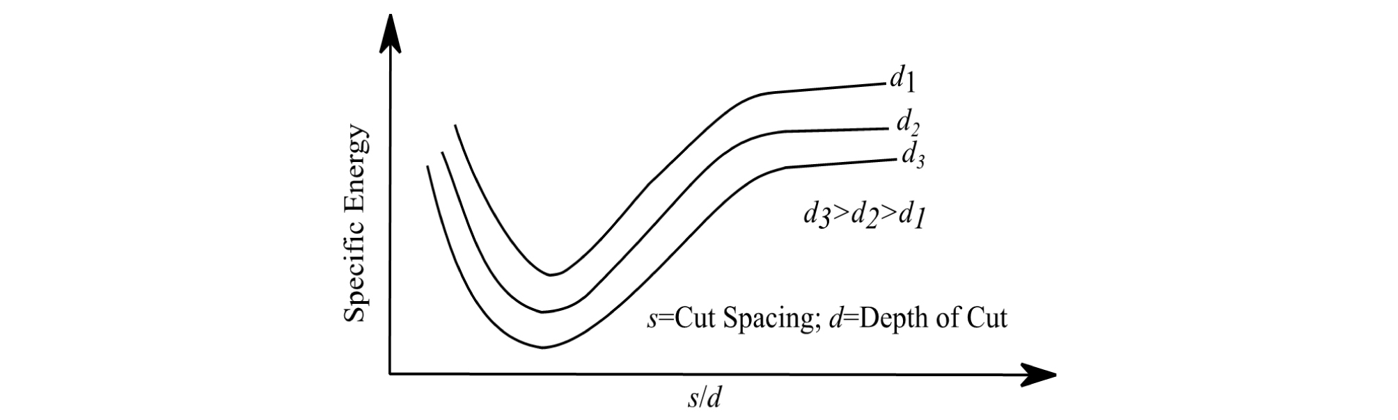
where IPR is instantaneous production rate in m3/hour, HP is the machine power in kW, is the efficiency of the machine, and SE is specific energy in kWh/m3 for full-scale cutting tools (disc, pick, etc.). HP is one of the machine`s capacity indices (e.q. thrust and torque) and is determined by the type of machine. On the other hand, the SE is affected by the cutting conditions (i.e. depth of penetration and cut spacing) and rock properties (i.e. strengths of rock, brittleness of rock, weakness plane, etc.). The SE is generally obtained from the full-scaled linear cutting machine (LCM) test, which is applicable to control the cutting conditions during the rock cutting by using full-scaled cutting tools (Jeong et al., 2011). The rock specimen of the LCM is typically made on an up to preconditioned piece of rock fixed in a stiff frame. The rock surface is conditioned so that it can be representative of the actual excavation surface. Depending on the desired experiment plan, the same cutting process is repeated using different spacings between the adjacent cuts and different depths of cut. Fig. 1 shows how SE reacts to changes in depth of cut and cut spacing. As the size of the cutter is the same as that of a real one, the results of this increasingly popular test bear minimum amount of uncertainty and can cover anomalous aspects of rock behavior that are rather inexplicable by its physical properties (Bilgin et al., 2013). The outcomes of this test may be used to either predict the performance of the mechanical excavators or enhance it through choosing the optimum cut spacing to depth of cut ratio (Bilgin et al., 2013). Eq. 2 shows how SE is determined based on the cutting force measured as a result of full-scale cutting experiment (Pomeroy, 1963; Roxborough, 1973):
| $$SE\;=\;\frac{FC}{Q\times3.6}$$ | (2) |
where FC is the cutting force in kN, Q is defined as yield or the volume of rock cut in unit length of cutting (m3/km), and SE is the specific energy in kWh/m3.
The full-scaled LCM directly measures the cutting force and the volume of cut rock during rock cutting process, but it requires a large amount of time and effort for preparing the full-scale specimen and performing the test (Jeong et al., 2012). To overcome the limitation of the test, the statistical analysis could be a reasonable way to estimate the SE. However, it is essential to establish the sufficient database and it is important to determine an appropriate statistical analysis method for estimation of SE.
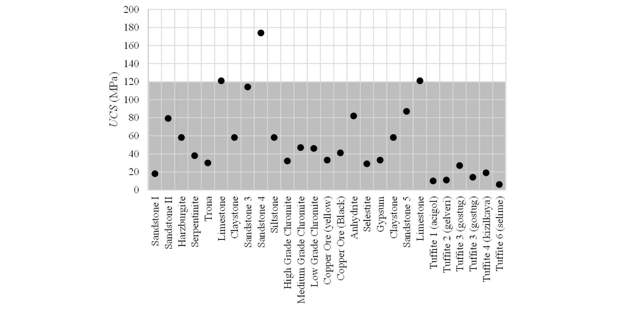
The purpose of this research, is to investigate the effect of intact rock properties, i.e. Uniaxial Compressive Strength (UCS) and Brazilian Tensile Strength (BTS), and operational properties, i.e. penetration depth (P) and cut spacing (S), on SE. Within the context of the present research, a total of 46 full-scale linear cutting test results, carried out using pick cutters having a conical shape, on various types of rock was used. The data was obtained from Copur et al. (2003), Balci et al. (2004) and Wang et al. (2018). Table 1 shows the descriptive statistics for the database used in this study. Copur et al. (2012) categorized the different types of cutters with respect to the maximum UCS values for the rocks to be cut. According to their classification, pick cutters may be used for cutting rocks with UCS values of up to 120 MPa. Fig. 2 shows the distribution of the UCS values used in this study over the range of application for pick cutters. For collecting all of the SE data used in this research, the cutting speed has been constant. It has been 12.7 mm/s for the data generated by Copur et al. (2003) and Balci et al. (2004), and 13 mm/s for the data generated by Wang et al. (2018). It should be added that, according to He and Xu (2016), for the constant cutting speeds in the range 4-20 mm/s, the effect of the cutting speed on SE may be safely ignored.
Table 1. Descriptive statistics for the data base used in this study
*1kWh=3.6MJ
After preliminary analysis of the established database, it was revealed that the conventional multiple linear regression (MLR) method is not capable of producing results with the desired accuracy (Eq. 3).
| $$SE=(2.77\times BTS)+(0.18\times UCS)-(2.779\times P)+23.721,\;R^2=76.7\%,\;MSE=52.94$$ | (3) |
| $$MSE=\frac{\sum_{i=1}^n\;(y_i-{\widehat y}_i)^2}n$$ | (4) |
where is the ith measured valued, is the ith predicted value, and n is the number of cases. Hence, a new genetic algorithm-based method called Gene Expression Programming (GEP) was implemented for data analysis (Ferreira, 2006). The advantage of GEP is that it can fit a highly accurate mathematical equation to the proposed data without any need to prior knowledge of the structure of the equation. That advantage makes GEP a better choice in comparison to artificial neural networks as they are intrinsically not capable of generating a differentiable equation for a function fitting problem.
In addition, GEP’s ability to autonomously evolve many different structures as candidate fitting functions makes it more favorable in comparison to optimization techniques (such as particle swarm optimization), which require a predefined function structure, such as y=alog(x)+bx+c, where a, b, and c are the optimizable parameters. Compared to genetic programming (GP), GEP has proven to be more efficient mainly because it is not prone to generating syntactically incorrect genes. Different genetic operators, such as mutation or recombination (see section 2, “Gene Expression Programming”, disturb the structure of chromosomes/genes in both genetic programming (GP) and GEP. While GP produces many instances of syntactically incorrect genes after application of genetic operators, GEP does not have that problem. Thus, the genes/chromosomes generated by GEP can evolve in a more efficient way using more diverse genetic operators than GP (Ferreira, 2006).
Çanakcı et al. (2009), Khandelwal et al. (2016), Faradonbeh et al. (2016), and Faradonbeh et al. (2017) showed the reliability and the high accuracy of GEP for solving an assortment of rock mechanics function fitting problems. Çanakcı et al. (2009) used GEP for predicting compressive and tensile strength of Gaziantep basalt from Turkey; Khandelwal et al. (2016) developed a model for predicting flow of air in a single rock joint; Faradonbeh et al. (2016) investigated the issue of predicting the rock flying distance in blasting operations in mines; and Faradonbeh et al. (2017) used GEP for predicting the performance of roadheaders.
2. GENE EXPRESSION PROGRAMMING (GEP)
GEP is a model/program generating evolutionary algorithm that can generate a population of chromosomes/individuals which are interpreted to mathematical equations and are visually expressed as tree structures. Chromosomes/Individuals are able to evolve through generations such that the best fitness for each generation is at least as good as that of the previous generation. For a function fitting problem, the “fitness” can be defined as one, or a weighted combination of, mean squared error (MSE), root mean squared error (RMSE), correlation coefficient (R), determination coefficient (R2), etc.
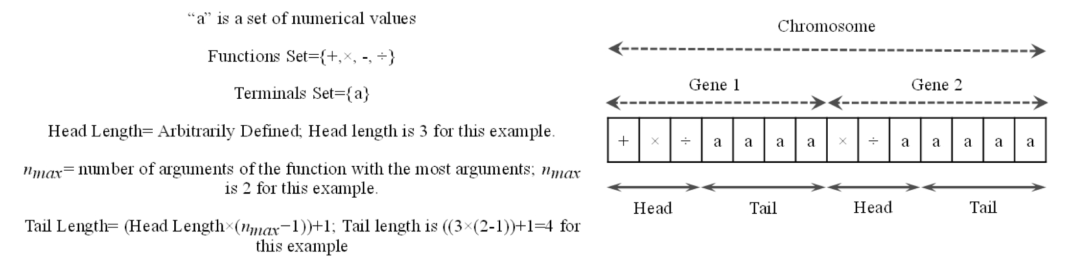
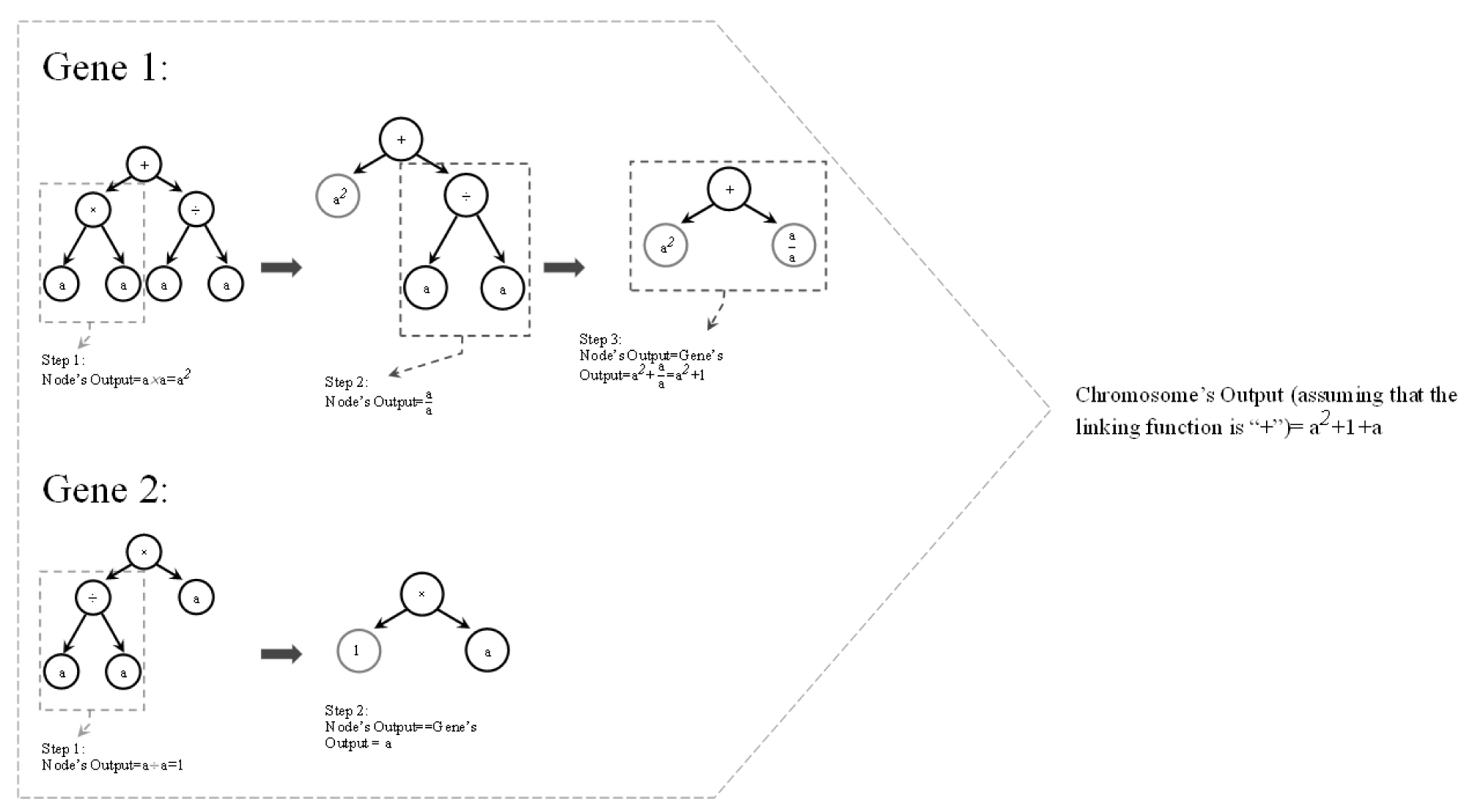
Each chromosome is consisted of a number of genes that are connected to each other by linking functions, which can be any mathematical operator such as addition, division, etc. Each gene has a head and a tail part. While the head can be constructed by a combination of members of functions set and terminals set, the tail part can only be consisted of terminals set subdivisions and feeds the functions in the head along with the terminals in the head itself. Functions and terminals sets are sets of mathematical functions, such as + or ×, and matrices of numerical values (e.g. values of UCS or BTS for all samples), respectively. The number of the units that form the tail part is determined based on the number of the units in the head, which is defined by the user. Fig. 3 shows a chromosome with two genes. In the expression tree, each circle is called a node. Fig. 4 shows the expression tree for the chromosome’s first gene, and its mathematical expression.
Similar to what happens in the nature, each generation, except the first one, is created by the children of the individuals of the previous generation. The individuals forming the first generation are generated randomly. Within each generation, the individuals are given the chance of reproduction proportional to their fitness. The evolution procedure is carried out by means of genetic operator(s), which can be one, or a combination of, mutation, inversion, different types of transposition, and different types of recombination. Evolution continues for a certain number of times or until the desired fitness is reached (Ferreira, 2006).
Depending on the mutation rate defined by the user, mutations are free to happen at any randomly selected unit across a gene, given that the resulting gene’s head can be consisted of functions and/or terminals while its tail is exclusively made of terminals (Fig. 5). Although it can take any value between zero to one, the mutation rate is usually set such that mutation happens for two units in each chromosome. It should be noted that mutation occurs within all of the individuals in the new generation (Ferreira, 2006).

Through the inversion process, a randomly selected sequence from head of a randomly selected gene is inverted. It should be noticed that the start and end points of the sequence are randomly selected within gene’s head. Inversion is restricted to only the head part of the genes (Fig. 6).

This restriction helps the structural form of the chromosome to be maintained. In other words, by limiting inversion to the head, there will be no risk of having a function at the tail of a gene. Across each generation, the number of the chromosomes that undergo inversion depends on the arbitrarily defined inversion rate (Ferreira, 2006).
Transposition operator, in simple words, randomly selects a piece of a gene and relocates it to a randomly selected place across the same chromosome. Three different types of transposition are defined in GEP algorithm. The first type is Insertion Sequence (IS) elements, and it is shown in Fig. 7. This type of transposition involves randomly selecting the start and ending positions (both positions can be either in head or tail of the gene) of a piece of a randomly selected gene and inserting that piece into the head of the same gene (except the first unit of the head or root) within the same chromosome. The second type is Root Insertion Sequence (RIS) elements, and it is shown in Fig. 8. The RIS element is the same as the first with two differences. The selected piece of gene in RIS elements type, unlike in IS elements, has to begin with a function and is inserted to the root of the same gene.


The third type, gene transposition (shown in Fig. 9), works in a larger scale than the other types. Gene transposition randomly selects a gene in a randomly selected chromosome and inserts it to the place of the first gene in that chromosome. Obviously, this operator makes a difference only for non-commutative linking functions.
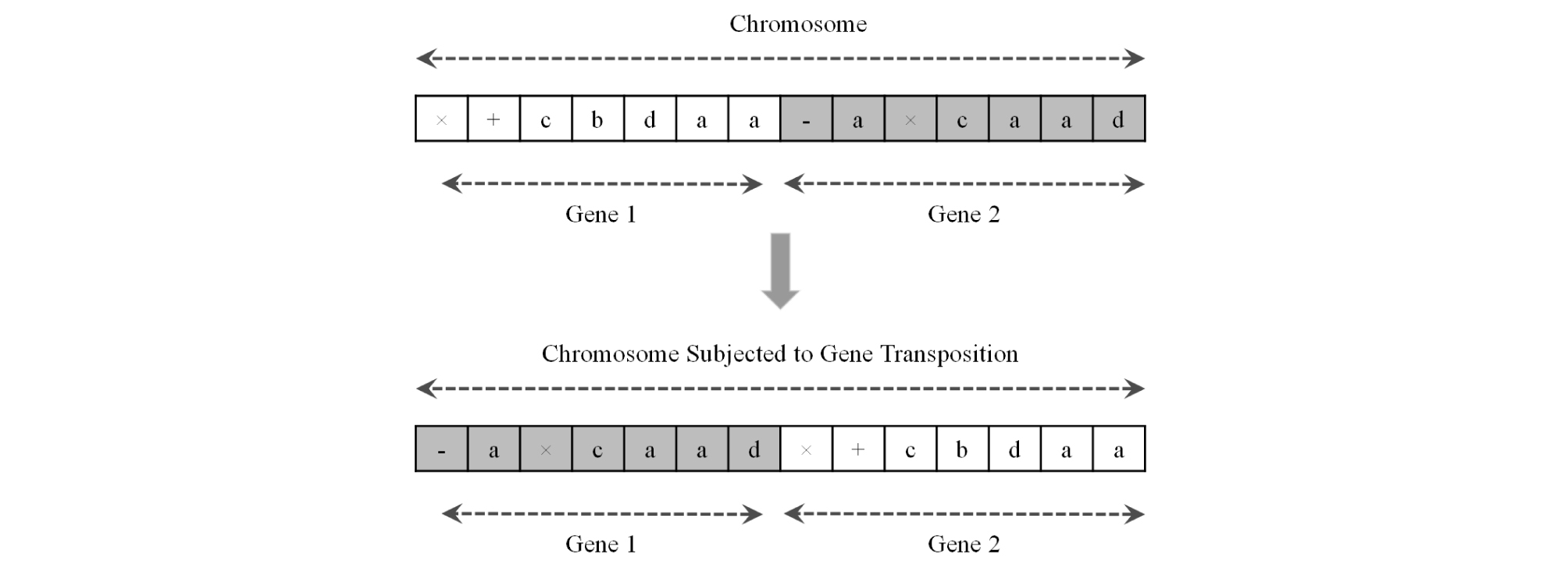
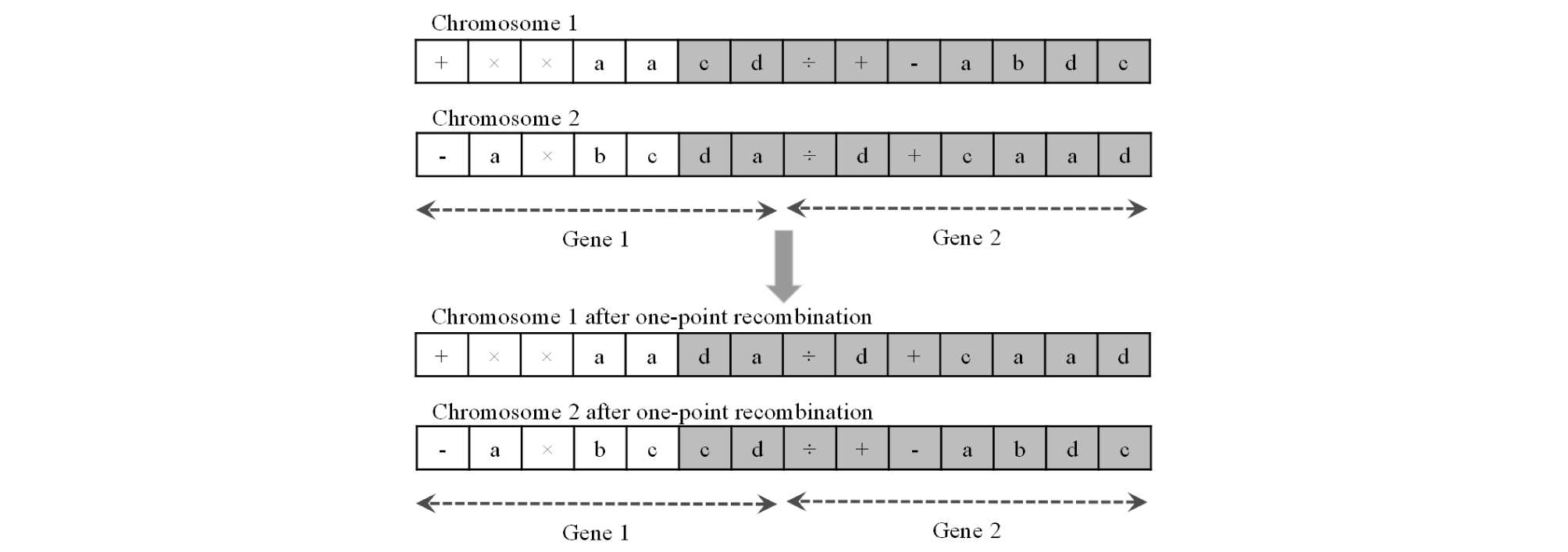
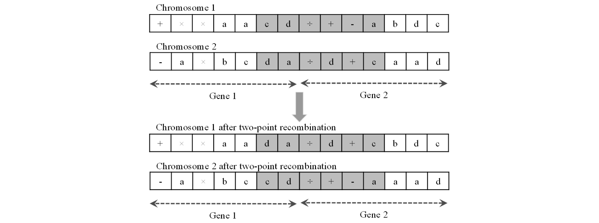
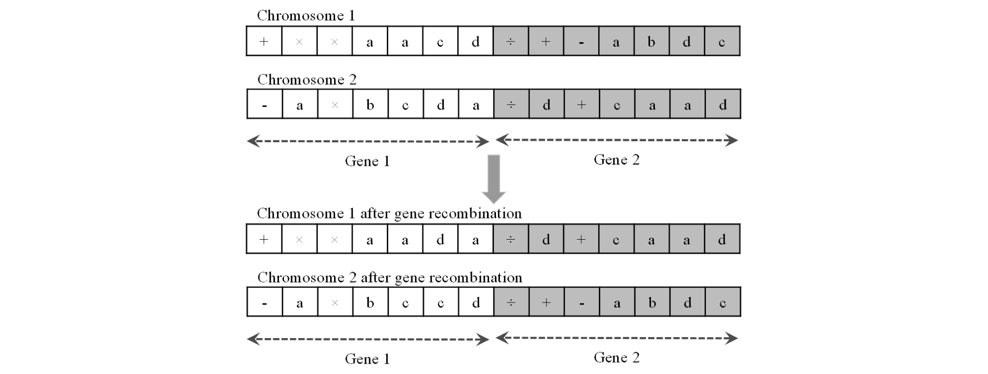
The number of times that each of the different types of transposition are repeated depends on the different types of transposition rates defined by the user (Ferreira, 2006). One-point, two-point, and gene recombination are the three different types of recombination that GEP algorithm uses as genetic operators. All of them involve randomly selecting two different chromosomes that are supposed to exchange some portions with each other. One-point recombination is carried out by randomly selecting a position along the chromosome and exchanging the parts of the chromosomes that start at that point and end at the end of the chromosome (Fig. 10). In two-point recombination, two positions are randomly selected along the chromosome and the portions limited to those two points are exchanged (Fig. 11). In gene recombination, whole randomly selected genes are exchanged between the two randomly selected chromosomes (Fig. 12). The number of times that each of the different types of recombination are repeated depends on the different types of recombination rates defined by the user (Ferreira, 2006).
The functions set used in this study is:
Functions Set= {+, ×, -, ÷, Power, ln, Exp, Sin, Cos, Tan}where “ln(x)” is the natural logarithm of the variable “x” and “Power” and “Exp” are defined as follows:
| $$\mathrm{Power}\;(x)=Ax^B,\;A\;and\;\;B\;\mathrm{are}\;\mathrm{real}\;\mathrm{numbers}$$ | (5) |
| $$\mathrm{Exp}\;(x)=Ce^{Dx},\;C\;and\;\;D\;\mathrm{are}\;\mathrm{real}\;\mathrm{numbers}$$ | (6) |
The terminals set used in this study is defined as follows:
Terminals Set= {UCS, BTS, P, S, S/P, Random Numbers}
where P, S, S/P are 46 × 1 matrices containing the values of cutting depth, cut spacing, and cut spacing to cutting depth ration, respectively. Random Numbers is also a 46 × 1 matrix the elements of which are a repeated numerical value. Although GEP is theoretically capable of generating some random integers in the genes’ outputs (please refer to Fig. 4, Gene 1’s output), Random Numbers are added to the terminals set in order to provide the algorithm with more freedom for creating models/genes with a wide range of numerical constants including integer and non-integer numbers.
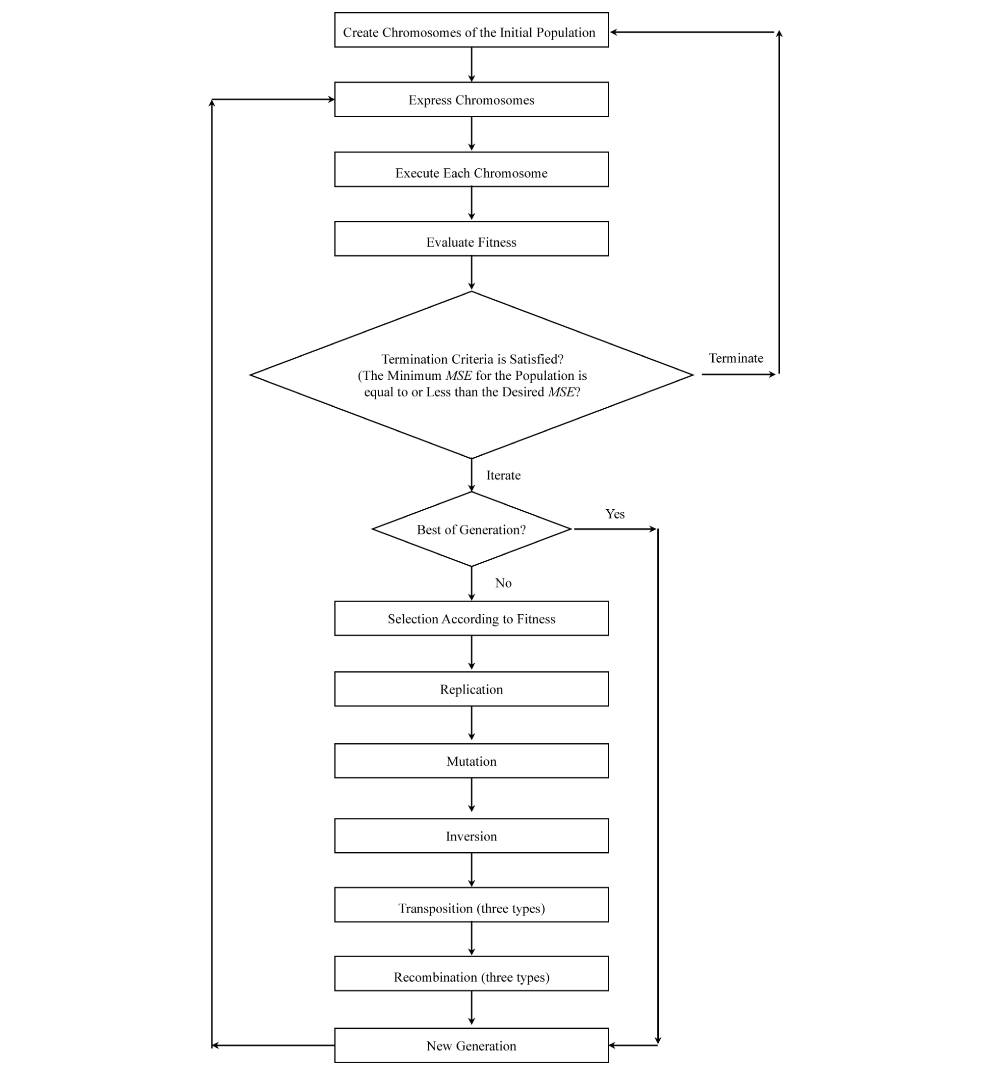
Finally, Fig. 13 shows the flowchart for the basic GEP algorithm according to the processes mentioned above.
3. PARTICLE SWARM OPTIMIZATION (PSO)
The presence of parameters such as A, B, C, D (Eqs. 5 and 6), and random numbers in genes creates an opportunity for application of an optimization method, which will lead to a more efficient evolution process for GEP. To take that opportunity, Particle Swarm Optimization (PSO) method was applied wherever those parameters appeared in a chromosome that had already reached an acceptable level of fitness using only GEP.
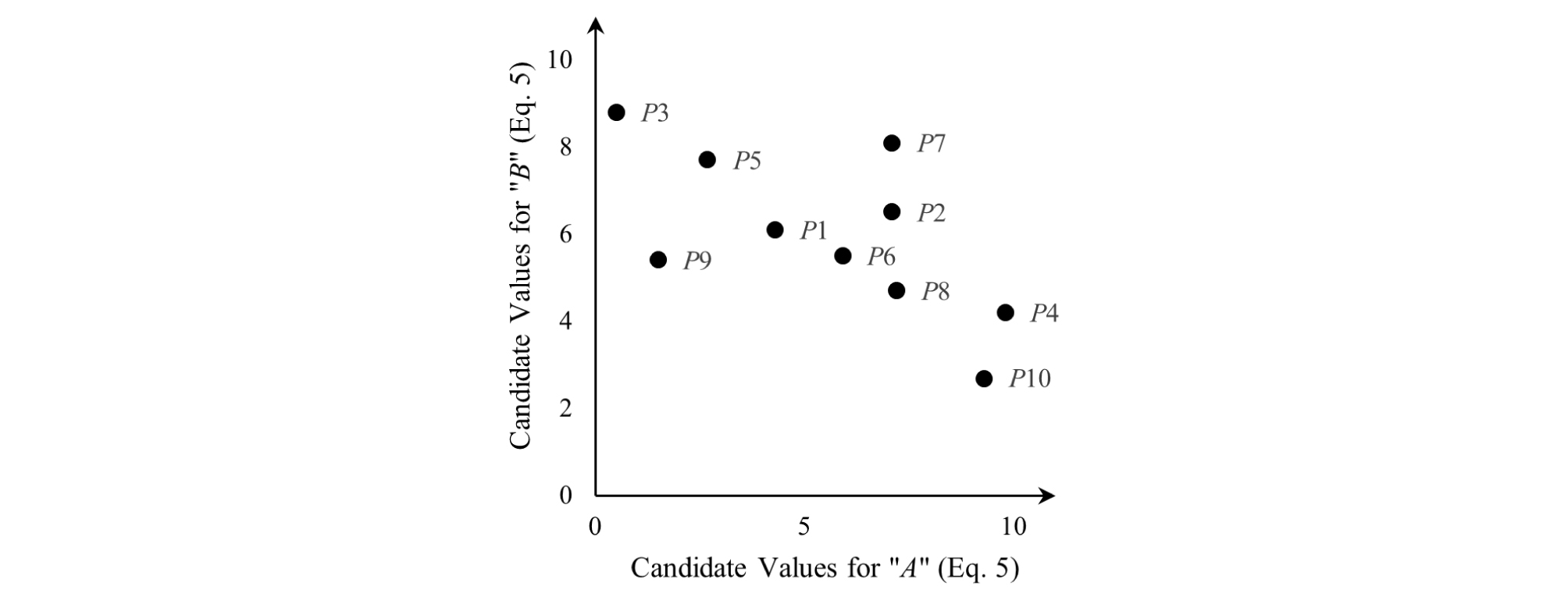
PSO is a population based optimization method inspired by movements of swarms such as a flock of birds or a school of fish that are in search of food or getting away from a threat, etc. (Kennedy and Eberhart, 1995). In this algorithm, a swarm of “particles/potential answers” is randomly distributed over a search space with number of dimensions equal to the number of optimizable parameters, e.g. A-B plane as the search space if the chromosomes contains only the “Power” function (Eq. 5). Each member is regarded as a candidate solution for the optimization problem at hand (Fig. 14).
Then, an iteration process starts. Through the process, the particles move over the search space with velocities defined for each of them according to their fitness. The search space is explored until the satisfactory answer is found or the maximum number of iterations is reached. “Fitness” can be defined depending on the user’s preference. In this research the fitness was defined by Mean Squared Error (MSE) (Eq. 4) associated with each swarm member/candidate solution. The velocity of each particle is updated with reference to the best particle in the population (the bird closest to the source of food or the lowest MSE among all of the particles) and the particle’s best (the closest each bird has been to the source of food through its moves or the lowest MSE the particle has experienced) within all of the iterations. In other words, in each iteration, a particle moves toward its own best and the best particle across all iterations which may be called Globally Best Particle. For a particle P(x,y) in x-y surface, the updated velocity is defined by the following equation:
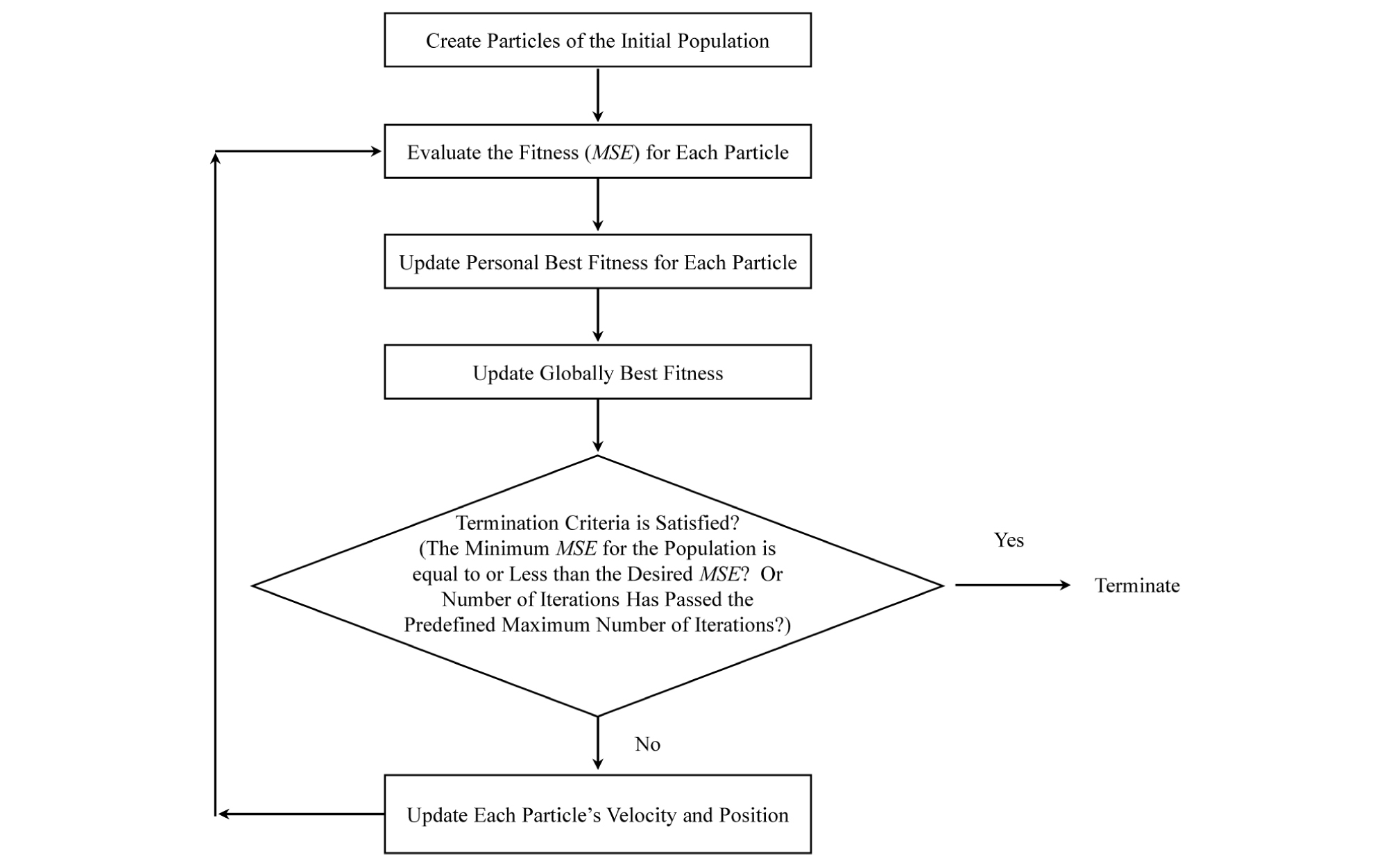
Where is the updated particle’s velocity for the current iteration, V is particle’s velocity in the previous iteration, Inertia is a user defined quantity that adjusts the extent of V’s impact on and is usually set to a number from [0.9-1.2], rand( ) is a random number from [0,1], LRPI is the Learning Rate for Personal Impact and it is a quantitative parameter recommended to be set as 2, LRSI is the Learning Rate for Social Impact and is also a quantitative parameter recommended to be set as 2 (Kennedy and Eberhart, 1995). The flowchart of PSO is presented by Fig. 15.
4. THE GEP-PSO ALGORITHM AND THE RESULTS
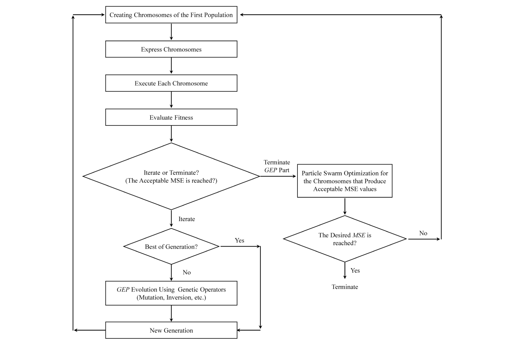
For the current research, a customized combination of GEP and PSO algorithms was used to find an equation that relates UCS, BTS, P, S, and S/P to SE. Fig 16 shows a flowchart of the algorithm used in this study. At first, GEP is applied. The evolution of GEP continues until it can find at least one equation/chromosome with acceptable associated MSE value, which is smaller than/equal to the MSE value associated with the equation generated by MLR (Eq. 3). At this stage, unless for the initial generation, the values for A, B, C, D (Eqs. 5 and 6), and Random Numbers are set to one. In this manner, an extra emphasis is put on finding the correct structure of the equation/chromosome rather than the best values for those parameters. When the acceptable MSE is reached, the chromosomes producing acceptable results are subjected to PSO optimization, to check whether the MSE can be improved to at least half of the MSE associated with MLR method (Eq. 3). In other words, structural evolution is carried out by GEP and PSO is used for numerical evolution of A, B, C, D, and Random Numbers. If the final goal is reached after optimization, the algorithm stops, otherwise it will start again by creating a new initial population for GEP (Fig. 16).
The difference between the basic GEP algorithm and the modified GEP algorithm is that all the genes are connected to each other by the same function, the genes outputs were used as terminals for another chromosome that uses the following functions set :
Functions Set= {+, ×, -, ÷}
In this manner, the algorithm is enabled to investigate all the different combinations of the genes and linking functions and select the best rather than merely adding or multiplying the genes outputs to calculate the final chromosome output. Fig. 17 shows the simple example of the difference between the chromosome`s output with dynamic and static linking functions. And Table 2 summarizes the settings used in the GEP-PSO algorithm.
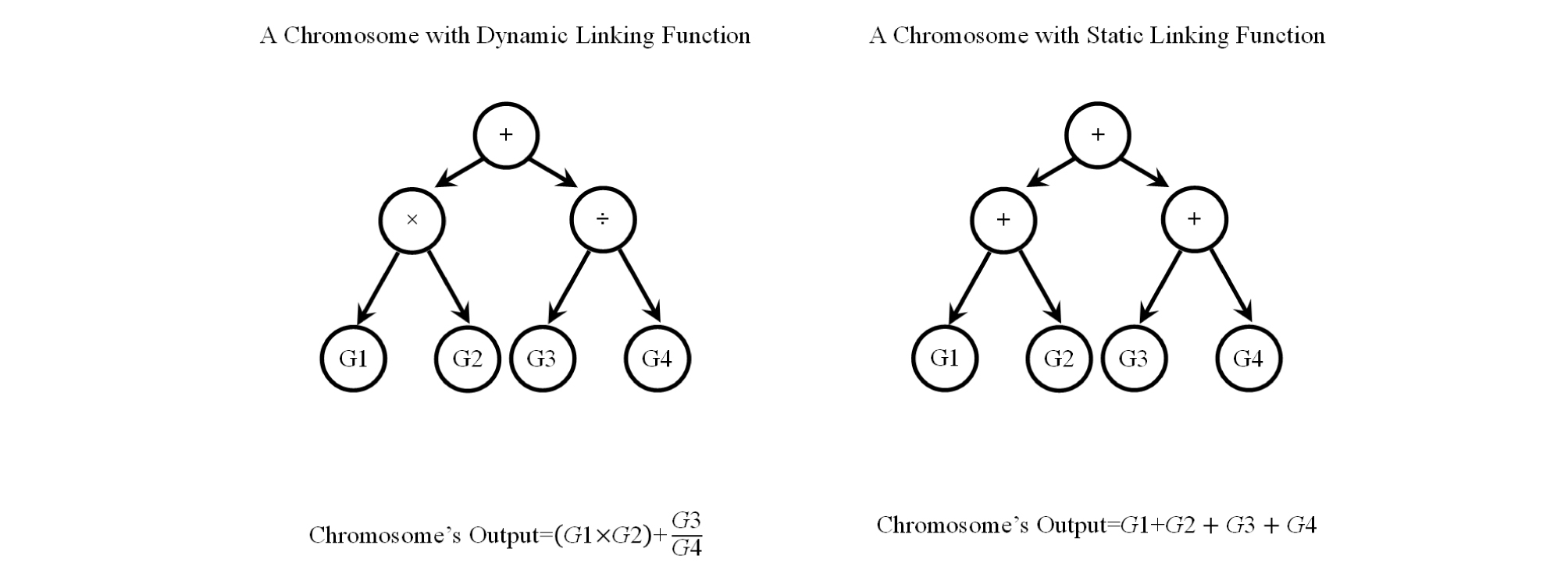
Table 2. The setting used in GEP-PSO code
The GEP-PSO algorithm, written in Matlab (2017), generated the following equation, which explains the variation in Specific Energy (SE) based on variations of UCS, BTS, depth of cut (P), and cut spacing (S):
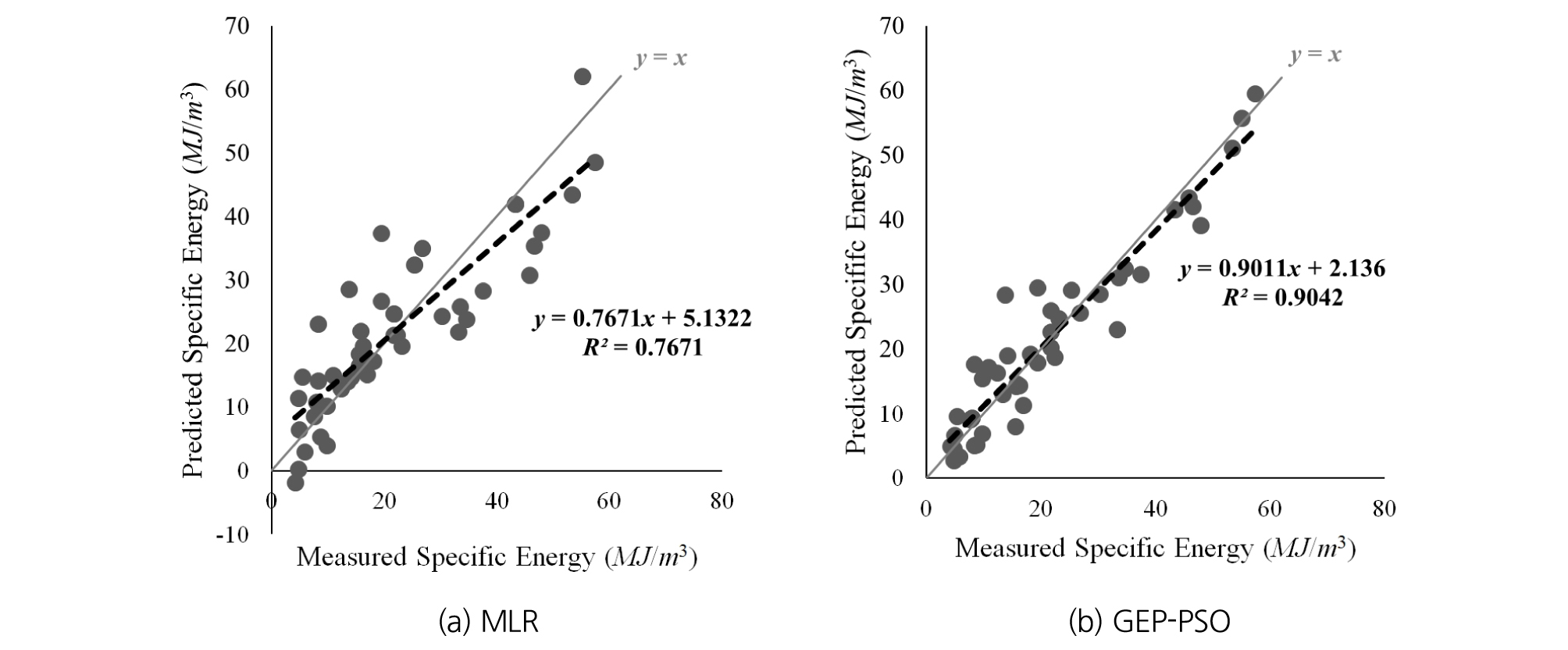
The results generated by the GEP-PSO code are compared against those generated by MLR in Table 3. As Table 3 shows, the MSE associated with MLR model is more than two times larger than the MSE associated with Eq. 8. In addition, the R2 value associated with Eq. 8, is about 0.13 higher than that of Eq. 3. Therefore, it may be concluded that the GEP-PSO algorithm generates a significantly better result in comparison to the conventional MLR method. The predicted SE values by the prediction models (from MLR and GEP-PSO) are visually compared against the measured values from LCM in Fig. 18.
Table 3. The results generated by MLR and the GEP-PSO code
5. THE EFFECT OF TIP, ATTACK, AND SKEW ANGLES ON SPECIFIC ENERGY
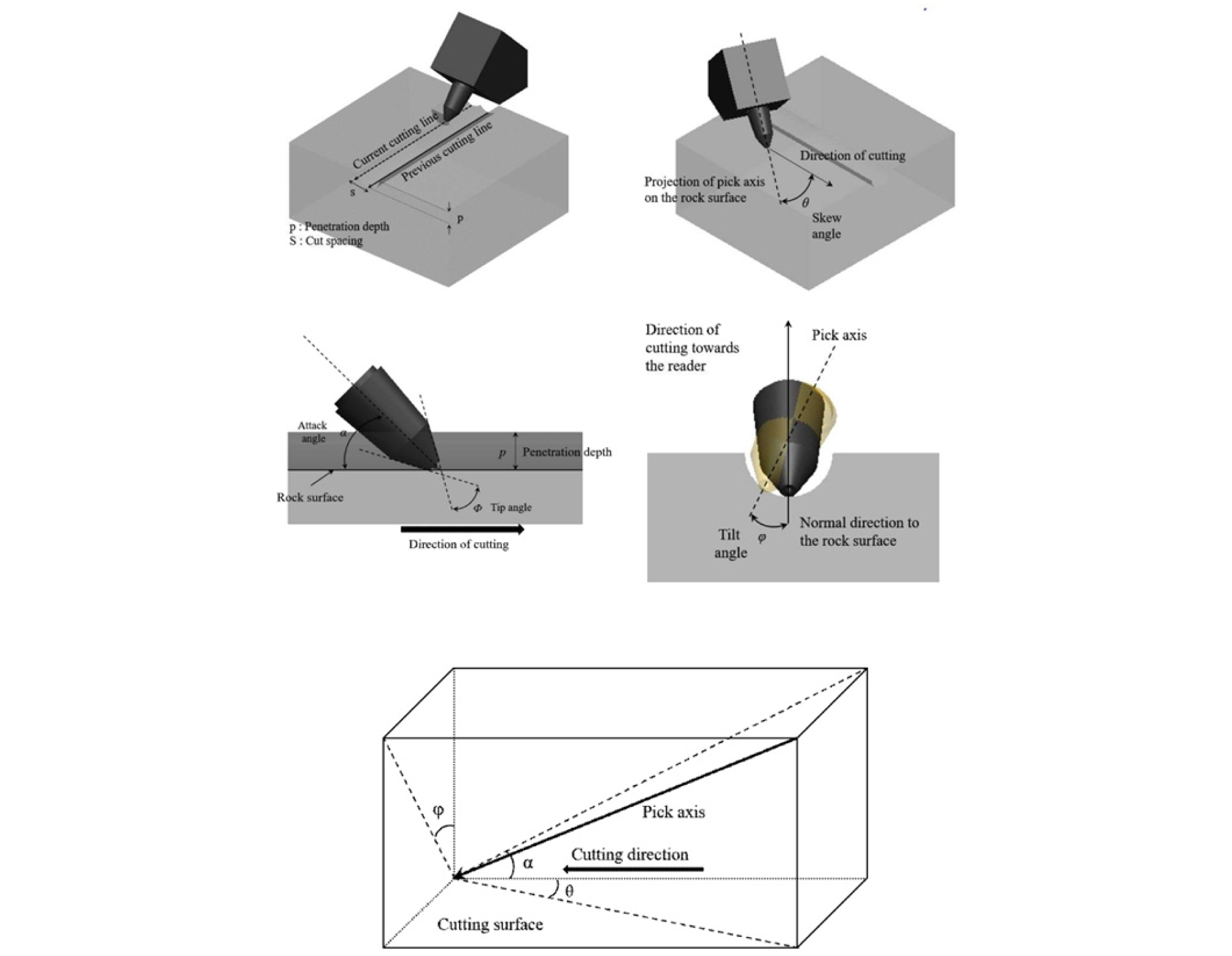
Besides the basic cutting parameters (i.e., penetration depth and cut spacing) considered in this study, many other parameters affect to the cutting performance of a pick cutter (Fig. 19). Jeong (2017) showed that the skew and attack angles have a significant effect on specific energy and cutting forces of a pick cutter. Changes in the values of those angles can change the area of the cutter in contact with rock. Therefore, they can consequently change the amount of stress transmitted to rock by cutters. Although a similar graph could not be provided for tip angle due to shortage of proper data, it can be assumed to have a similar effect on SE as tip angle can similarly change the area of the cutter in contact with rock. Therefore, it can be inferred that if the data, over which a SE prediction functions is fitted, contains a variation of those angles, the generated prediction models will be more reliable. In the present research, the effect of those angles is not taken into consideration because the established database is generated using only one value for each of the angles (Tip angle =80°, Attack angle=55.5°, and Skew angle=0). Based on the provided explanations, at least a part of the error associated with the developed GEP-PSO model (Eq. 8) can be attributed to not using those angles in the database that fed the algorithm.
6. CONCLUSIONS
In conclusion, it may be stated that the developed GEP-PSO model is capable of predicting SE values with a dramatically higher accuracy than the conventional multiple linear regression technique. The proposed model and approaches may be used as a useful tool for estimating the cutting performance and the operational parameters of the mechanical excavators. Because it may be helpful in reducing the efforts for the full-scaled LCM tests to find the preferable design parameters of the mechanical excavators (i.e., P, S and SE). The range of application for the developed model is limited to the ranges of the data it has been trained with (minimum and maximum values for UCS, BTS, P, S, and S/P shown in Table 1 while tip angle, attack angle, and skew angle are 80, 55.5, and 0 degrees, respectively).
Considering the significant effect of tip, skew, and attack angles on SE, for the future work, it will be added more testing data to the database used in this study in order to investigate the effect of variations in those angles on SE. It is hoped that, for the future work, the GEP-PSO algorithm can be improved such that even more accurate models with less sophisticated mathematical equation can be reached.
